
October 5, 2026
Sizing Multi-Site Capacity with
Loss-of-Load Probability
SUMMARY
Cerbrec builds AI inference availability across a set of simple sites rather than inside one heavily redundant building. A Tier I site has no backup generator or duplicate power and cooling paths, so it costs less to build and less to run, and it goes down more often. The question is how much that matters once capacity is spread across sites.
The answer comes from Loss-of-Load Probability (LOLP): how often the tenant’s demand exceeds the capacity still running. Demand is modeled as a daily cycle times random variation times occasional bursts. Three findings follow:
- 01
A small set of Tier I sites can beat one Tier III site.
In every demand profile modeled, two to four Tier I sites lose less service to facility outages than a single Tier III building. Spreading wins because a site outage rarely meets a peak: with demand averaging 30%, losing one site for a short period almost never causes a shortfall.
- 02
The availability target sets a downtime budget, and the budget sets repair urgency.
With typical inference demand on five sites, each site can be down about 140 hours a year and still deliver four nines, nearly five times the Tier I benchmark. Repairs can be scheduled rather than dispatched as emergencies, which is where operating cost falls.
- 03
Bursts can exceed all installed capacity, in any facility.
That overload is a capacity-planning question, not a facility failure, and it affects Tier I and Tier III equally.
Why build redundancy across sites
A Tier III data center buys availability inside one building; Cerbrec buys it across buildings. The industry’s long-cited benchmarks put a Tier I site at 99.671% (about 29 hours of downtime a year) and a Tier III site, with N+1 redundant power and cooling, at 99.982% (about 1.6 hours).
Cerbrec treats the whole site as the redundant unit instead:
- Graceful degradation. Losing one of four Tier I sites costs 25% of capacity. Losing the Tier III site costs 100%.
- Lower cost per site. Tier I sites need no backup generator and no duplicate power and cooling paths.
- Independent risk. No two sites in a Site Set share a utility territory, so one grid event cannot take down two sites.
Demand-aware sizing
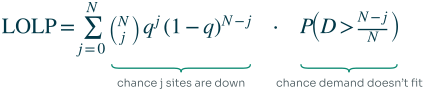
The question a Site Set has to answer is how often the tenant’s demand exceeds the capacity still running. That is Loss-of-Load Probability (LOLP), and it combines two ingredients.
How site outages combine. Say a Site Set has N sites, each down a fraction q of the time (q = 0.0033 for a Tier I site). The chance that exactly j of them are down at once is:

That is q to the power j for those j sites being down, times (1−q) for each of the others being up, times the number of ways to choose which j. Each extra simultaneous outage is roughly 300 times less likely than the last.
Whether demand fits. Capacity is the tenant’s installed IT power, and D is demand as a share of it. With equal sites, losing j of N leaves (N − j)/N running, and demand fits unless D is above that.
Putting them together:
Sites do not have to be the same size. With Pᵢ the IT power at site i, the general form sums over every combination of sites up and down:

The largest site matters most: the states where it is down leave the least power, so a lopsided layout shows up directly as a higher LOLP.
One term dominates. Because two simultaneous outages are so much rarer than one, LOLP is close to the one-site-down term: N sites that could fail, times q, times the chance demand exceeds what the rest can carry. That gives a simple test. A Tier I set beats a single Tier III site when:

With four sites, demand needs to exceed 75% of capacity less than about 1.4% of the time.
Modeling inference demand
Inference demand is modeled as three factors multiplied together:

- Daily baseline. Average level b with a daily swing of ±a.
- Random variation. Lognormal noise with mean 1 and spread σ, which widens demand around the baseline without moving its average.
- Burst multiplier. Equal to 1 most of the time. For a share p of the time it multiplies demand by a burst factor of typical size M.
This produces the shape real inference traffic tends to have: a broad middle, a steeper falloff toward the daily peak, and a tail from bursts that is fatter than a smooth curve would give.
Bursts can exceed all installed capacity. A burst landing on a daily peak can ask for more than 100% of what the tenant installed. That happens in any facility, Tier I or Tier III, and no site layout prevents it. This paper therefore reports two figures:
- Facility-caused shortfall: demand within installed capacity that goes unserved because sites are down. This is what site design controls.
- Total shortfall: facility-caused shortfall plus time when demand exceeds all installed capacity.
Scenarios: Tier I sets against a Tier III site
Four illustrative tenants, all averaging 30% utilization, differ in how their demand moves. For each, the chart compares facility-caused availability on Tier I sets of 1 to 10 sites against a single Tier III site.
Four Tier I sites beat one Tier III site in every demand profile
Nines of demand served within installed capacity, by number of Tier I sites. All profiles average 30% utilization.
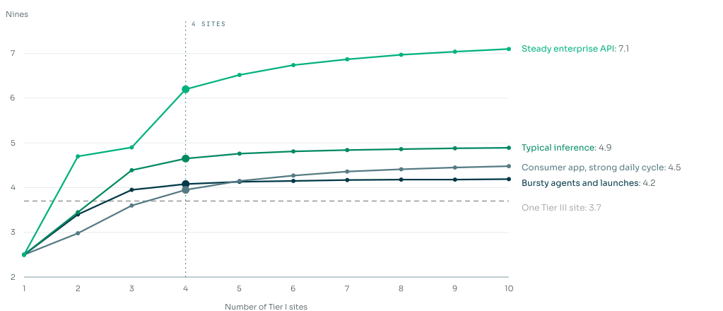
Four Tier I sites beat the Tier III site for every profile, by 0.2 nines for the most volatile consumer traffic and by 2.5 nines for a steady enterprise API. Steadier demand keeps gaining from extra sites; bursty demand levels off past four, because its bursts mostly overshoot all installed capacity rather than the capacity a site outage removes.
| Demand profile | Daily swing | Bursts | Time above installed capacity | Tier III | 4 Tier I sites | 6 Tier I sites | Total incl. overload: Tier III / 4 Tier I |
|---|---|---|---|---|---|---|---|
| Steady enterprise API | ±30% | 0.2% of time at 1.5× | under 0.001% | 3.7 | 6.2 | 6.7 | 3.7 / 6.0 |
| Typical inference | ±50% | 1% at 1.8× | 0.04% | 3.7 | 4.7 | 4.8 | 3.2 / 3.4 |
| Consumer app, strong daily cycle | ±80% | 1% at 1.8× | 0.12% | 3.7 | 4.0 | 4.3 | 2.9 / 2.9 |
| Bursty agents and launches | ±50% | 3% at 2.5× | 0.6% | 3.7 | 4.1 | 4.2 | 2.2 / 2.2 |
Availability in nines. The Tier III, 4-site and 6-site columns are facility-caused; the last column adds time when demand exceeds all installed capacity. Random variation spread is 0.10 to 0.20 across profiles.
Once overload is counted, the bursty profiles sit near the same ceiling in either design: about 2.2 nines for bursty agents, set by demand exceeding installed capacity 0.6% of the time. Site design cannot raise that ceiling; capacity planning and the platform levers in the companion paper can.
How much downtime each site can afford
The same math run in reverse gives each site a downtime budget: the most it can be down while the Site Set still meets the target. Using the one-site-down approximation:
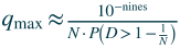
The budget grows with every site added and shrinks as demand gets more volatile.
Hours of downtime each site can have per year while the Site Set delivers four nines of facility-caused availability:
| Demand profile | 3 sites | 4 sites | 5 sites | 6 sites | 8 sites |
|---|---|---|---|---|---|
| Steady enterprise API | 84 h | 279 h | 395 h | 564 h | 863 h |
| Typical inference | 55 h | 96 h | 137 h | 164 h | 194 h |
| Consumer app, strong daily cycle | 12 h | 26 h | 39 h | 51 h | 69 h |
| Bursty agents and launches | 26 h | 35 h | 39 h | 41 h | 43 h |
For reference, the Tier I benchmark is about 29 hours a year and Tier III about 1.6 hours. Wherever the budget is above 29 hours, a Tier I site has room to spare.
Downtime is outages times time to restore. A site’s unavailability is roughly how often it fails, λ outages a year, times how long each takes to fix:

With typical demand on five sites, a site that has four outages a year can take about 34 hours to restore each one: next-day dispatch instead of a one-to-four-hour emergency response. Dispatch urgency, on-site staffing and local spares are where a Tier I site saves operating cost, and the downtime budget says how far that can go.
Servers have a budget too. Server failures trim each site’s capacity by a small, predictable amount. With typical demand on Tier I sites, each server can be unavailable about 2.5% of the time, roughly 9 days a year, and the Site Set still delivers four nines. A failed server can wait for the next scheduled visit rather than an urgent replacement.
What it means for the SLA
The SLA should commit to facility-caused availability: serving the tenant’s demand up to its installed capacity.
- Overload is excluded. Demand above installed capacity is a capacity-planning question. It is measured and reported to the tenant, but it does not count toward a breach.
- The demand profile sets the site count. Four sites beat a Tier III site for every profile modeled here. Steadier tenants get more from extra sites; bursty tenants gain little past four.
- More nines are a design choice. A tenant who wants more can add sites, even out site sizes, or install capacity above its peak, and LOLP shows what each buys.
- Overload is where the platform helps. Shared headroom across models, autoscaling and spilling bursts to interruptible capacity reduce overload; the companion paper, Telemetry-Driven Availability, covers that math.
Assumptions and limits
- Independent site failures. Separate utility territories cover power, but a shared control plane, network or software stack can fail everywhere at once. One such hour a year caps availability near 99.99%.
- Benchmark availability figures. The 99.671% and 99.982% figures are long-cited industry benchmarks for Tier I and Tier III, not certified measurements.
- Fast failover. Every minute spent rerouting counts as lost. Inference sessions holding in-memory state may drop during that time.
- Server failures as a uniform trim. The scenarios leave server failures out; the server budget treats them as a small, even reduction in every site’s capacity, which holds when each site has many servers. Outage counts per year are illustrative, and time-to-restore figures should be recalculated from each site’s measured failure history.
- Planned maintenance. Tier I sites must go offline for maintenance. A site down for planned work counts as one of the outages the design absorbs, so maintenance is limited to one site at a time.
- Illustrative demand profiles. Real sizing should fit the three-factor model to the tenant’s measured utilization.